Antenna Tutorial¶

The Antenna Module enables parametric measurements by varying the position of the Device Under Test (DUT) and acquiring its frequency response. The application captures the data, calculates antenna gain, saves the results, and visualizes the plots. Measurements can be reloaded from saved data, so tests do not need to be repeated unnecessarily.

Sample datasets are available in the data/Antenna folder.

Average Measurement Time

Scan \(\theta\) (\(1^{\circ}\) step) with fixed \(\phi\): ~16 minutes
Scan \(\theta\) (\(3^{\circ}\) step) with fixed \(\phi\): ~8 minutes
Scan \(\theta\) (\(5^{\circ}\) step) with fixed \(\phi\): ~6 minutes
3D scan (\(3^{\circ}\) step for both \(\theta\) and \(\phi\)): ~20 hours, (~380 MB for 201 frequency points)
3D scan (\(5^{\circ}\) step for both \(\theta\) and \(\phi\)): ~8 hours
- Note only half \(\theta\) scan may be needed for full 3D pattern, cutting the total time in half.

Theory¶

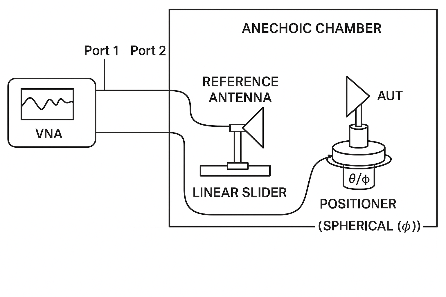
ARES is built to test antennas assuming the following setup:

Port 1 of the VNA is connected to the reference antenna
Port 2 of the VNA is connected to the antenna under test (AUT)

Foundational Equations¶

Friis Transmission Equation:

\[ \frac{P_r}{P_t} = G_t G_r \left( \frac{\lambda}{4 \pi d} \right)^2 \]

Where:

\(P_r\): Received power
\(P_t\): Transmitted power
\(G_t\): Transmitter Antenna Gain
\(G_r\): Receiver Antenna Gain
\(\lambda\) Wavelength
\(d\): Distance between transmitter and receiver

Which can be expressed in dB scale as:

\[ P_r^{[dB]} = P_t^{[dB]} + G_t^{[dBi]} + G_r^{[dBi]} + 20 \log \left( \frac{\lambda}{4 \pi d} \right) \]

The Free Space Path Loss (FSPL) factor is given by:

\[ FSPL = 20 \log\bigg( \frac{\lambda}{4 \pi d} \bigg) \]

The ratio of received to transmitted power will be the measured magnitude:

\[ S_{21} = \frac{P_r}{P_t} \]

Gain Comparison Method¶

In the gain comparison method (i.e., two antenna method), the reference antenna gain is known. Hence, we can solve the Friis transmission equation with this assumption and express it in terms of the measured S-parameters \(S_{21}^{[dB]}\), calculated \(FSPL\), and reference antenna gain \(G_{REF}^{[dBi]}\).

\[ G_{DUT}^{[dBi]} = S_{21}^{[dB]} - FSPL - G_{REF}^{[dBi]} \]

Gain Transfer Method¶

In the gain transfer method (i.e., one antenna method), the DUT and reference antenna are identical (\(G_t^{[dBi]} = G_r^{[dBi]}\)). Hence, we can solve the Friis transmission equation with this assumption and express it in terms of the measured S-parameters \(S_{21}^{[dB]}\) and calculated \(FSPL\).

\[ G_{DUT}^{[dBi]} = \frac{S_{21}^{[dB]} - FSPL}{2} \]

Performing the Measurement¶

Calibration¶

To get started, calibrate the Vector Network Analyzer (VNA) at the measurement plane, where the reference antenna and DUT will be connected. Set your frequency range and number of points (or step size) as desired before calibration.
Using an eCal is highly recommended, as shown in the following demonstration.

Connect to the Instruments¶

Select the relevant instrument VISA addresses in each dropdown of the Instruments tab.
Select None: NA for the instruments that will not be used.
Follow the Instrument Database Tutorial for detailed information on how to edit the user-defined instrument database.
Once all the addresses have been populated, click on Connect at the bottom to establish a connection to each instrument and Disconnect to clear all connections.

The Measurement Delay (s) can be modified at any time before the measurement starts. This value is the time in seconds to wait between setting all the instruments and capturing the data.

Load Reference Antenna Data (for Gain Comparison Method)¶

For the Gain Comparison Method, the reference antenna gain needs to be loaded using the same data format as measured antennas.

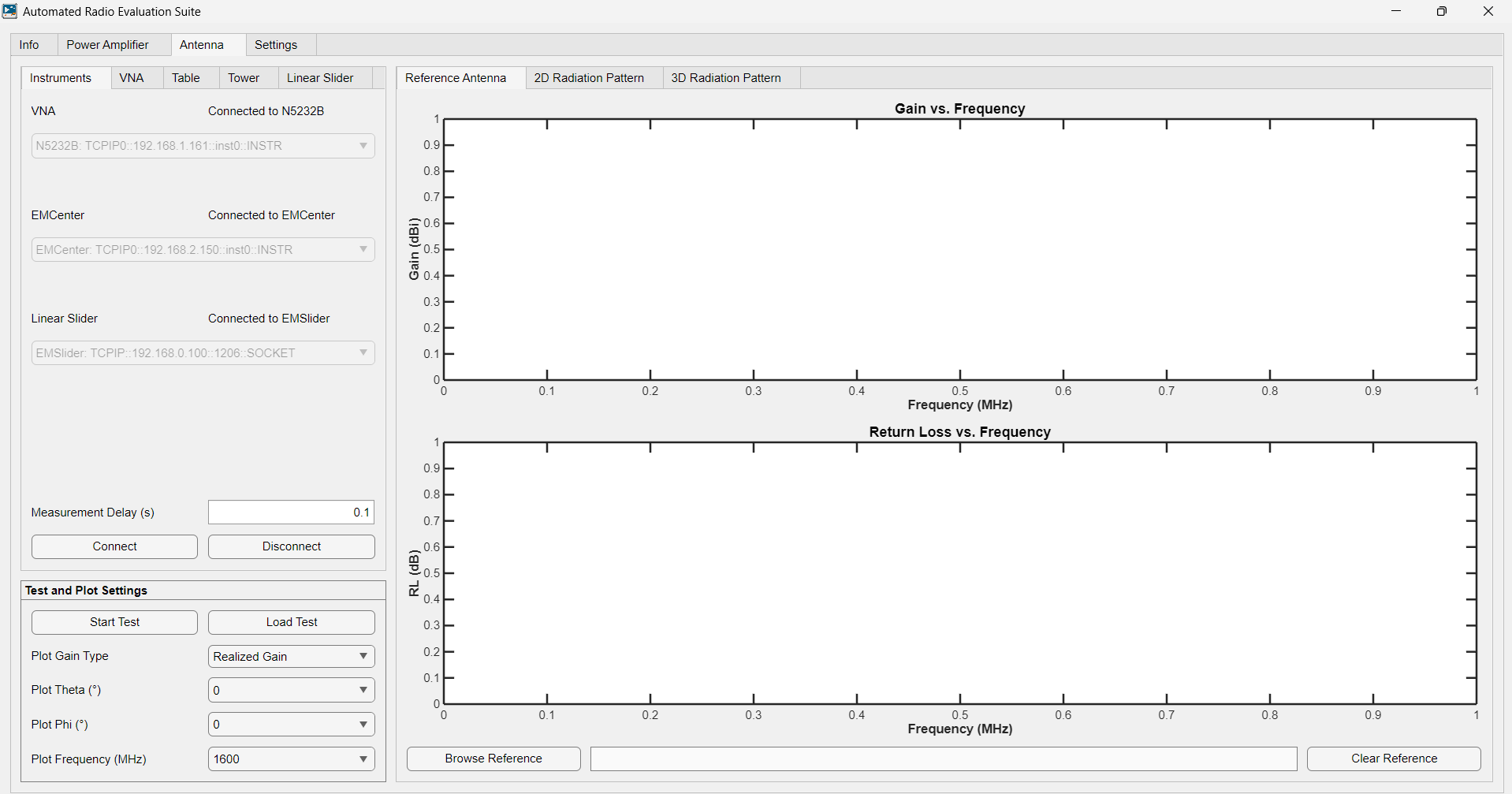
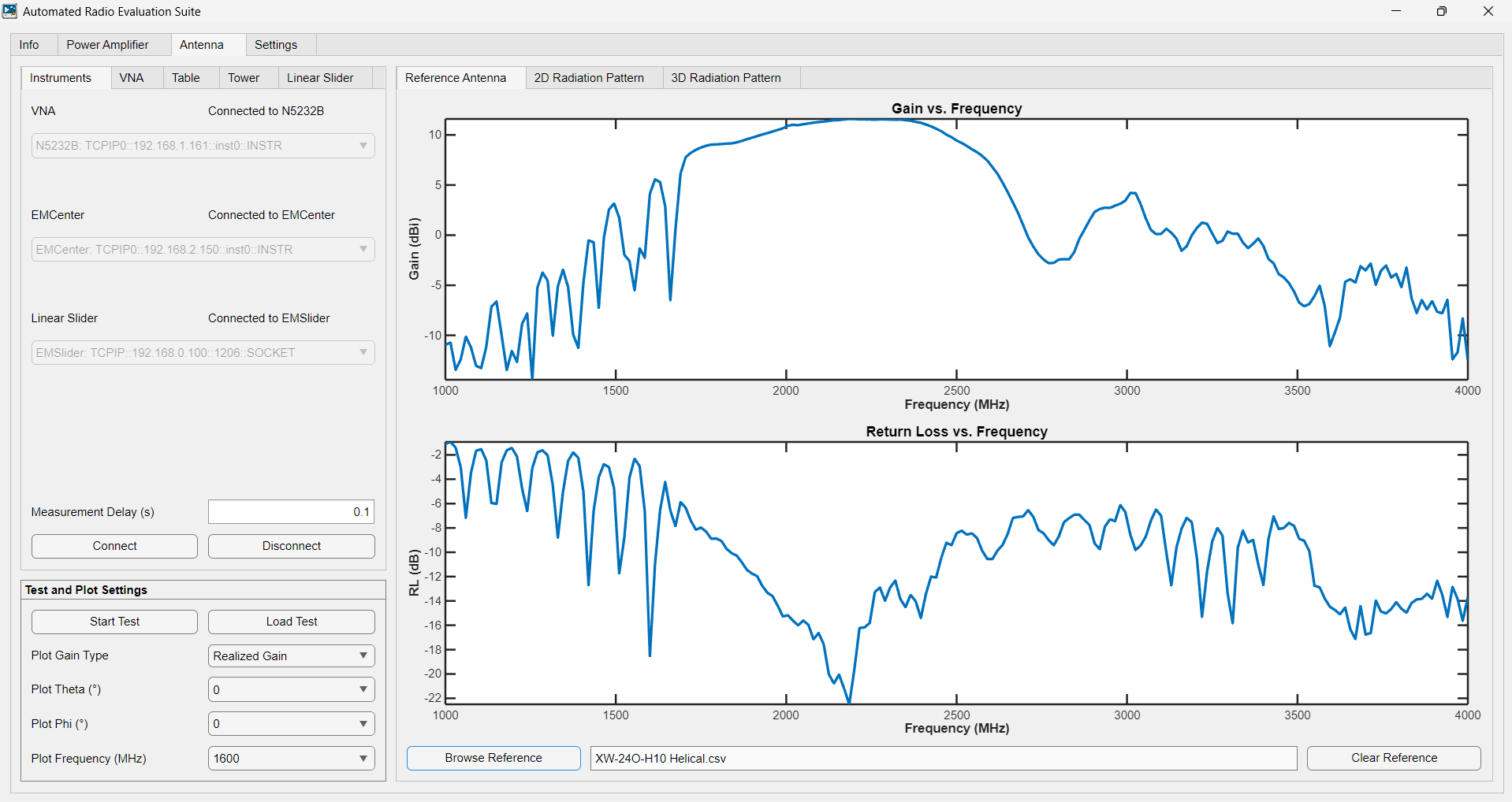
In the Reference Antenna window, click Browse Reference and select the file containing your reference antenna data.
Only the boresight gain (\(\theta = 0\), \(\phi = 0\)) is required from the reference antenna.
After loading, the boresight gain and return loss magnitude over frequency will be plotted in the results view.
The filename of the loaded reference data will be shown below the plots.
To remove the file, click Clear Reference.

Configure the VNA¶

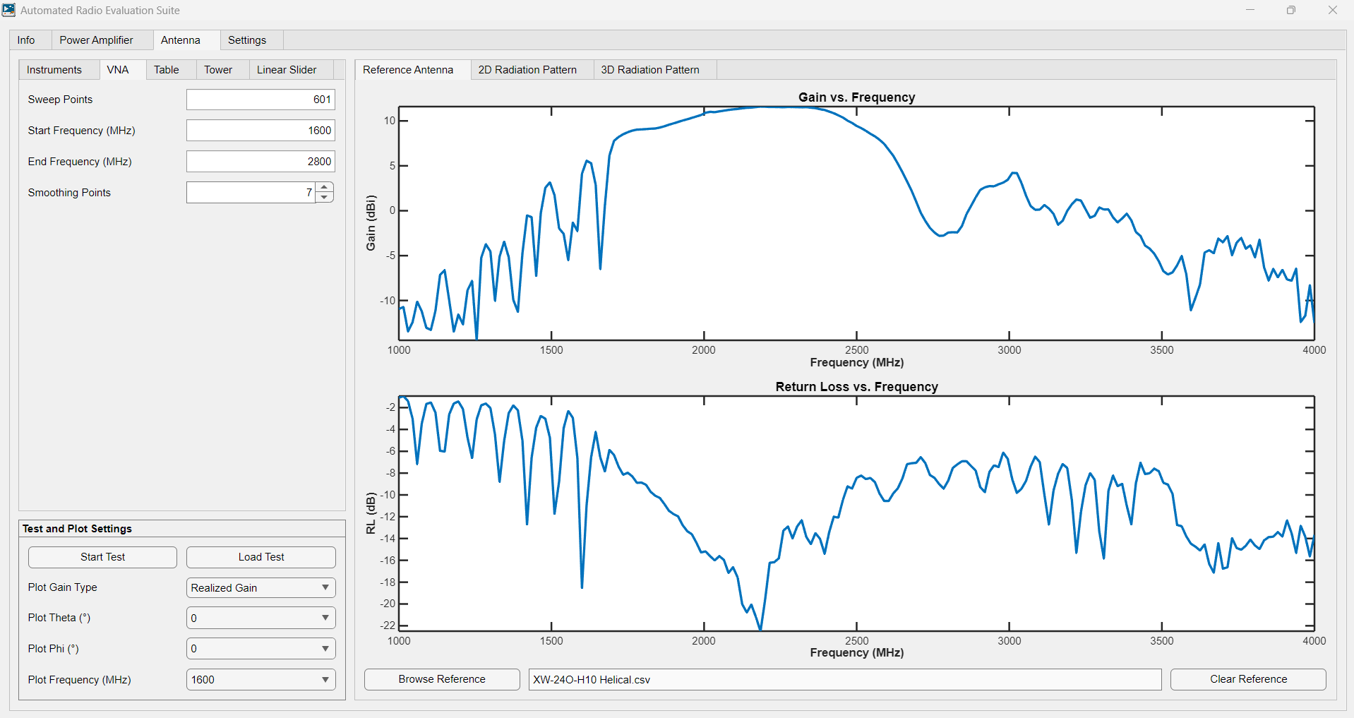
Use the VNA tab to review and adjust Vector Network Analyzer (VNA) settings. When the VNA is connected, its current configuration is automatically loaded into the app. If you modify key parameters such as Sweep Points, Start Frequency, or Stop Frequency, the existing calibration may no longer be valid.

To avoid invalidating the calibration, it is recommended to perform the VNA calibration before connecting to the VNA and then leave the loaded values unchanged. Keep in mind that the frequency and power ranges are constrained by the capabilities of the connected instrument.

Optionally, the app can apply smoothing to the VNA data using a moving average filter with the given number of samples. This is controlled via the Smoothing Points setting. If set to zero, smoothing is disabled.

Configure the Turntable (\(\theta\) axis)¶

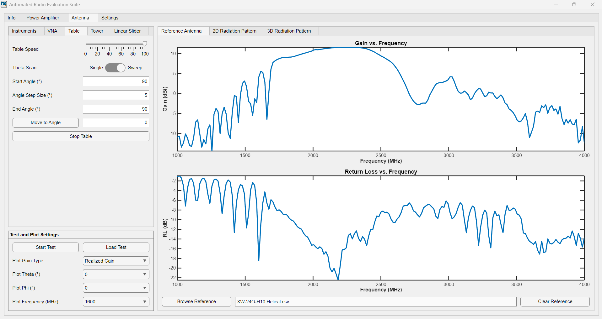
Use the Table tab to set up \(\theta\)-axis rotation for antenna measurements.

To configure the turntable:

Select either a static or parametric sweep.
Adjust the Table Speed using the slider.
Enter appropriate Start Angle, Angle Step Size, and Stop Angle values.

Note: Software inputs range from \(-180^\circ\) to \(180^\circ\), but the table is configured to operate from \(0^\circ\) to \(360^\circ\). The software automatically translates angles accordingly.

To control the turntable manually:

Enter a desired target position and click on Move to Angle.
To stop the movement at any time, click on Stop Table.

Configure the Tower (\(\phi\) axis)¶

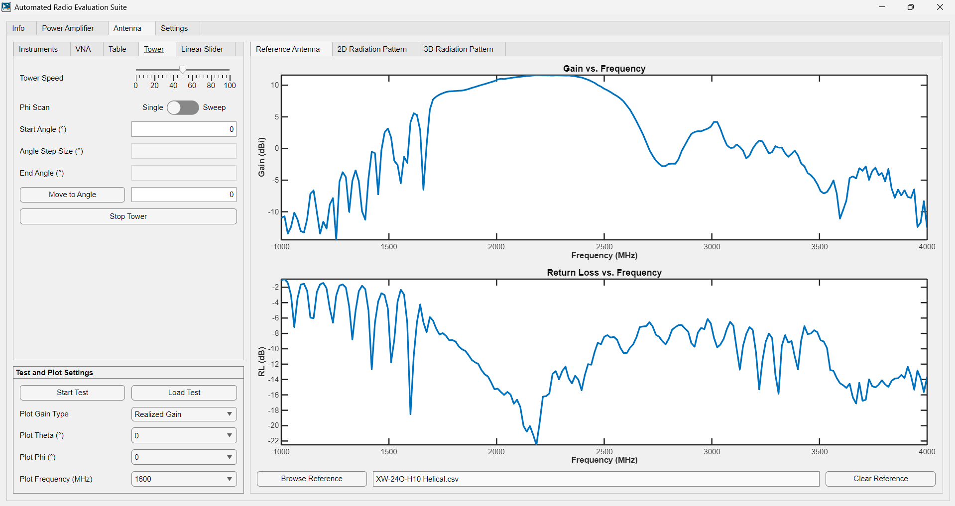
Use the Tower tab to set up \(\phi\)-axis rotation for antenna measurements.

To configure the tower:

Select either a static or parametric sweep.
Adjust the Tower Speed using the slider.
Enter appropriate Start Angle, Angle Step Size, and Stop Angle values.

Note: Software accepts inputs between \(-180^\circ\) and \(180^\circ\).

To control the tower manually:

Enter a desired target position and click on Move to Angle.
To stop the movement at any time, click on Stop Tower.

Configure the Linear Slider¶

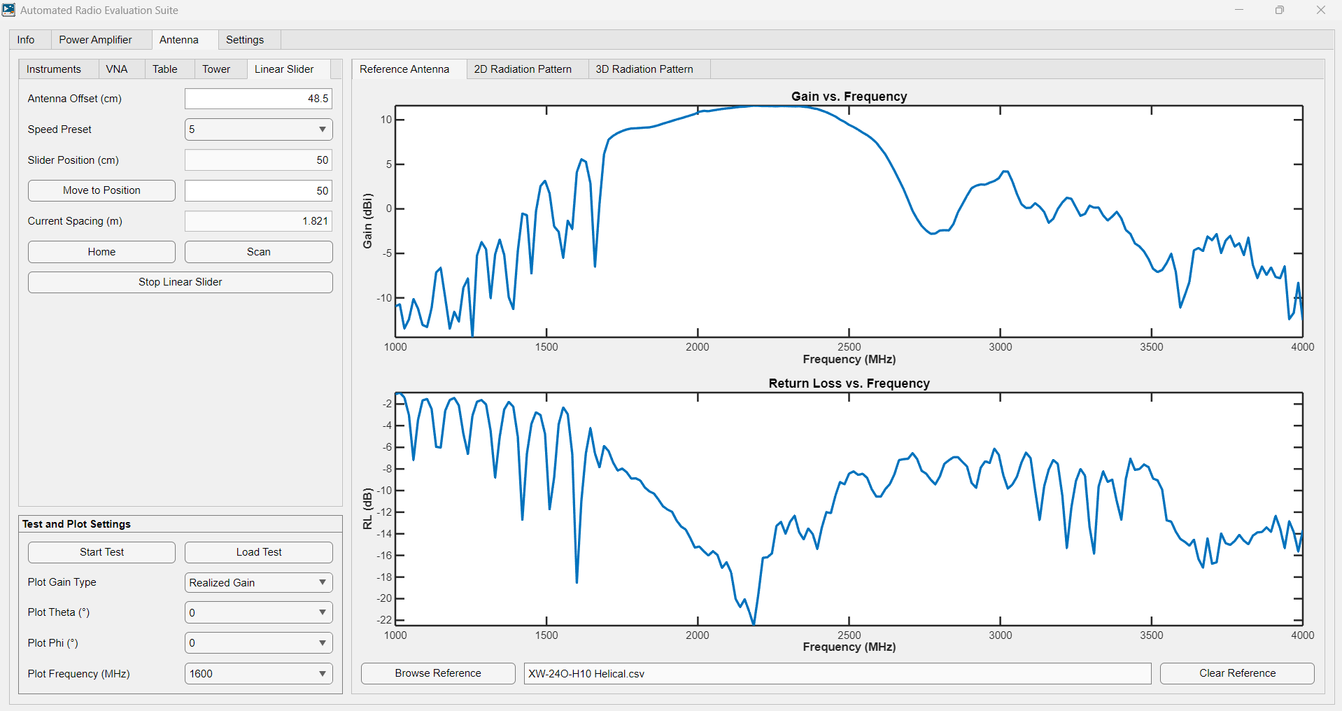
Use the Linear Slider tab to control antenna spacing and movement along the rail.

To configure and operate the slider:

Set the Antenna Offset in centimeters, which accounts for the physical length of both the DUT and reference antennas relative to the mounting fixtures.
Choose a Speed Preset for how fast the slider moves.
Enter a target Slider Position and click Move to Position to move the antenna.
Use the Home, Scan, or Stop buttons to control motion directly.

Live displays include:

Slider Position – the real-time position of the slider, given in centimeters.
Current Spacing – the calculated antenna separation, factoring in the slider position and antenna offset, given in meters.

Run the Test and Plot the Results¶

After verifying all configuration settings, click Start Test to begin the measurement.

During the test:

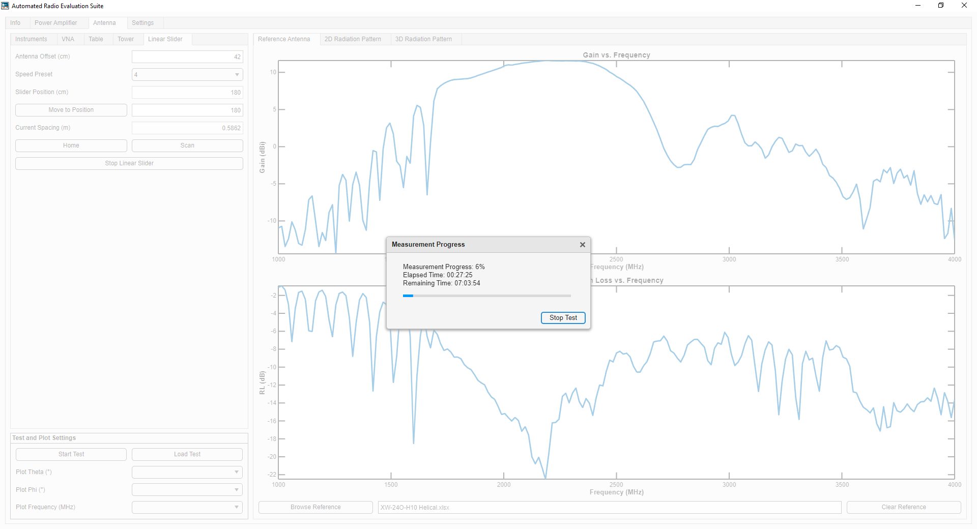
A progress window will show elapsed time and estimated completion time.
To terminate the test, press the Stop Test button on the progress window.
Once the test is finished, a prompt will appear to save the results.

After saving your results:

The measurement data is automatically loaded and visualized by ARES.
To view previous results, use the Load Test button.

2D Radiation Pattern Results¶

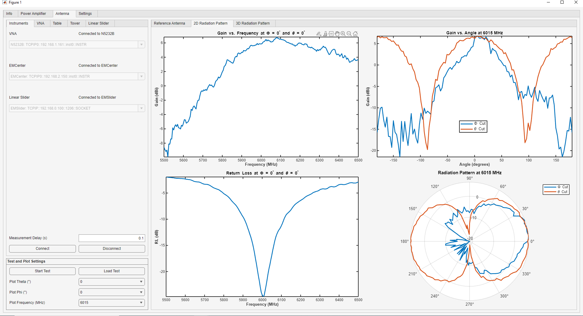
The 2D Radiation Pattern window displays:

Realized gain vs. frequency
Return loss vs. frequency
2D cartesian and polar plots based on the selected value from the Gain Type, Frequency, \(\theta\), and \(\phi\) dropdowns.

3D Radiation Pattern Results¶

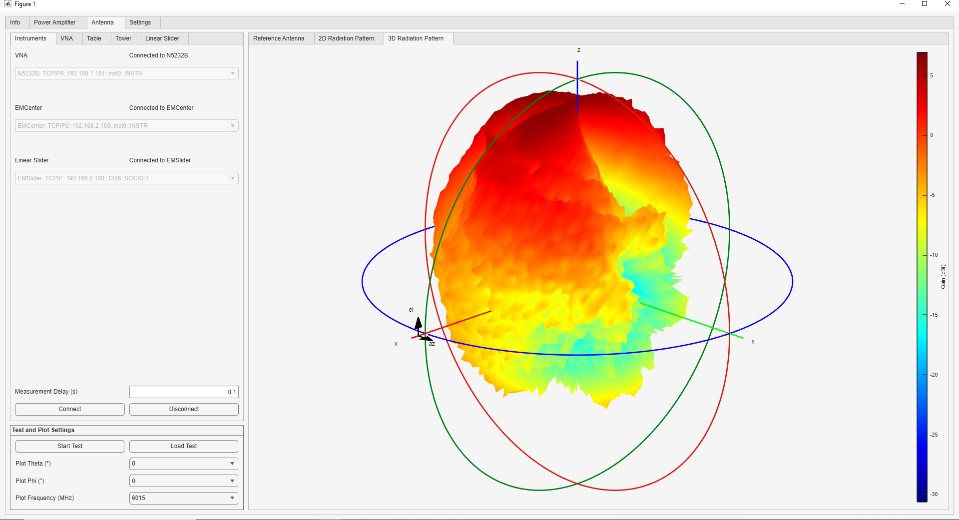
The 3D Radiation Pattern window displays:

Full 3D gain pattern for the selected frequency and Gain Type.